Mathematical models and statistical models

I suppose I started thinking about this really hard in the early days of the COVID-19 pandemic. I’m not sure it’s something we articulate well; the difference between a mathematical model. A mathematical model is meant to capture the science of a phenomenon in mathematical terms. A statistical model is meant to “fit” data and account for the uncertainty; but doesn’t necessarily explain the science. And there are certainly plenty of examples where you’re fitting a statistical model to estimate the parameters of a mathematical model. There’s a brilliant article from 2019 in Nature Communications which sets out the arguments in an advanced form. Here, I’m going to attempt to set out what I think are the key issues using more accessible (if slightly artificial) examples.

Ordinary Linear Regression (a Taylor approximation)

The first example is a fictional bivariate data set. The figure below these data (blue dots) with a “line of best fit” (red). This is the basic building block of more realistic statistical modelling.

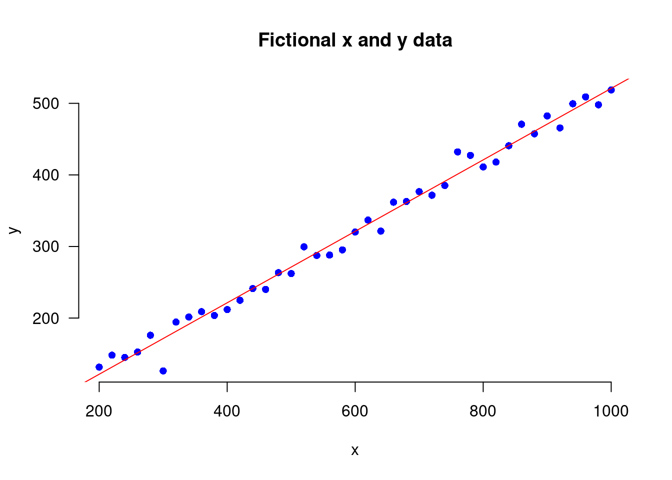
But what is this “line of best fit”? Bill Venables has pointed out that we can think of a standard linear regression as a Taylor approximation to the science, the mathematical functions that explain in scientific terms the mechanisms that lead from one variable to the other. If we assume \(Y\) is a random response variable, \(\boldsymbol(x) = (x_1, \ldots x_p )\) is a vector of \(p\) potentially explanatory variables and \(Z\) is a standard random normal variable. A conventional linear regression model is specified as:

\[Y \approx \beta_0 + \sum_{i=1}^p \beta_j (x_i - \bar{x}_{i}) + \sigma Z\]

If we write a first order Taylor approximation we get:

\[Y \approx f(\bar{x}_0,0)+\sum_{i=1}^p(\bar{x}_0,0)(x_i-x_0) +f^{p+1}(\bar{x}_0,0)Z\]

where the terms correspond. Note that we have assumed mean-centering; but in the absence of mean centering the additional terms would be wrapped into the intercept. We could extend this by adding first order interactions and single variable quadratics resulting in a second order Taylor approximation. So really, when we fit a statistical model, we are claiming that in the real world we have some function that relates one set of variables to the other:

\(Y = f(x, Z)\)

As we don’t have the functional form of \(f(\cdot)\), we claim we can still learn from a local approximation. Note the big caveat, locally approximate. Conversely, a mathematical model is meant to capture the science.

Logistic growth model

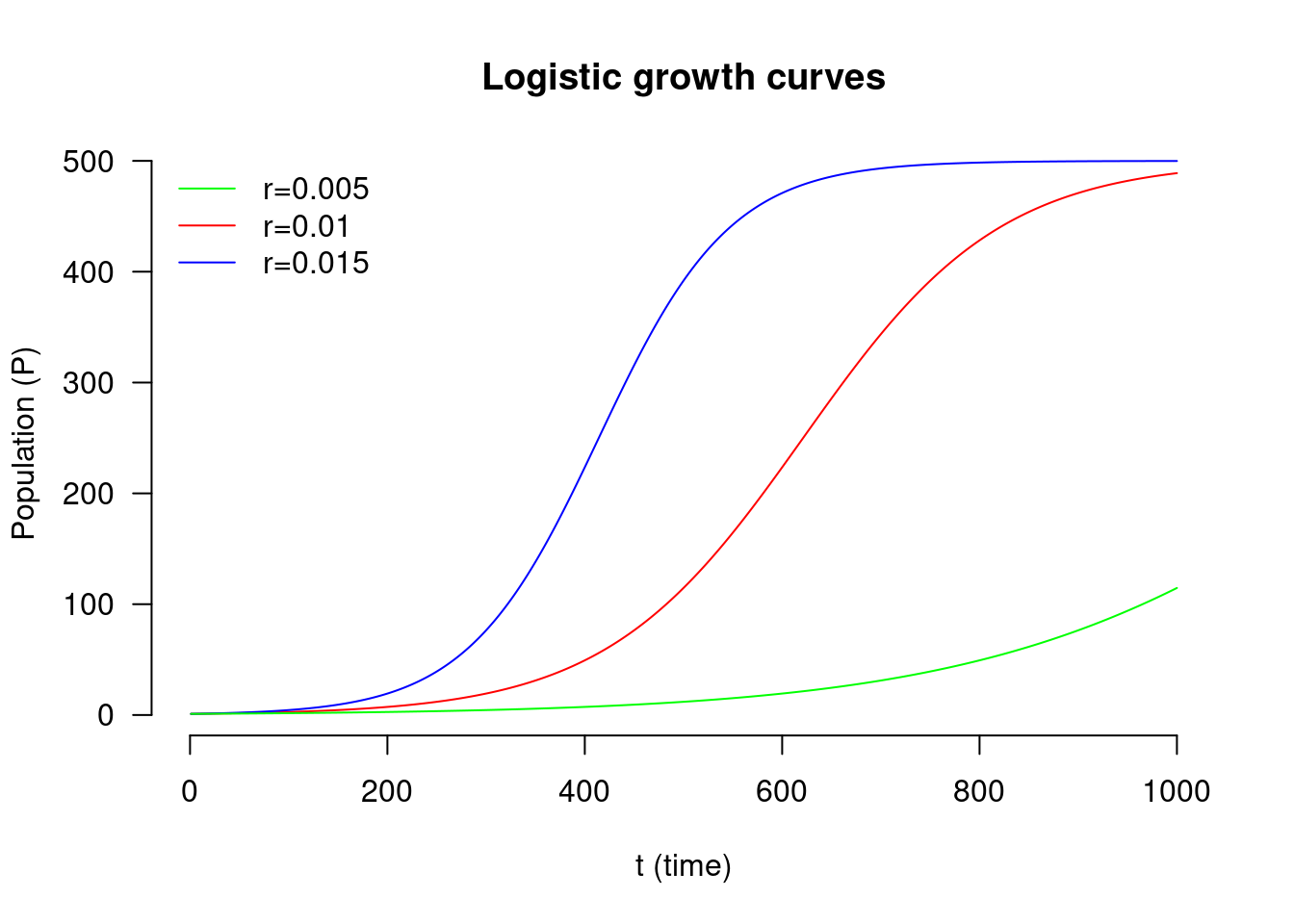
One simple example of a mathematical model is the Logistic growth model. In the early stages it models expontial growth, but this slows as the population reaches the carrying capacity of its environment. At least that’s the science claimed by the model. Let \(N\) denote the size of a population and \(t\) denote time. I want to know how the size of the population changes with time, which we can write as \(\frac{dP}{dt}\) (change in population size by change in time). The standard logistic growth model says that this rate of growth is equal to:

\(\frac{dP}{dt} = rP\left( 1 - \frac{P}{K} \right)\)

where \(r\) is the growth rate and \(K\) is the carrying capacity. The idea is that represents some fundamental state of nature. If I have an organism (a mould) and an environment (some left over Pizza) the mould will have an intrinsic rate of growth \(r\) in that environment and the Pizza will support a population of size \(K\). If we think a little about that formulae, at the start of our growth phase, \(P\) will be small relative to \(K\) so \(\frac{P}{K}\) will be small (close to zero) and so the term inside the bracket will be close to \(1\). This tells us that the growth, the change in Population by time will be close to \(rP\). As the population gets close to the carrying capacity then \(\frac{P}{K}\) will be close to \(1\). So the term inside the brackets will the close to \(0\) and the growth rate will be \(r \times P \times\) small value, i.e., it will be small. This is meant to describe a fundamental state of nature.

Assumptions

So one massive and under-rated part of either paradigm of modelling, statistical or mathematical, is that both require us to make a large number of assumptions. If we have structured the math model correctly, it can make statements that are universally correct. If we have structured the statistical model in an acceptable way, we can make statements about relationships between observed variables. Both approaches to modelling have their place. But both models rely on assumptions. Neither model is innately true. Therefore the assumptions should be challenged and checked rigorously. I think this blog is an attempt to start thinking about assumption checking in models.

Transport modelling

So the two examples given above are clearly toy examples. But these issues; the reliance on assumptions apply very much in models that are used in real life. Here is one attempt to explain some of the problems with the mathematical (economic) models used in transport modelling.